A retail investor would be forgiven for assuming that there are really only two assets classes one should consider for personal investments: equities (stocks) and fixed income (bonds). Wherever you look, these two asset classes dominate the financial landscape. All robo-advisors and most personal advisors implement a mix of bonds and equities for the portfolios of their clients. The idea behind this mix is simple: bonds are low risk and will earn you a marginal return, while equities are riskier and will be the real engine of returns in good times. In bad times, bonds will rise, mitigating some of the losses of your equity portfolio: it's been long known and accepted that stocks and bonds have a negative correlation. Tying this strategy together is periodic rebalancing, taking money off the table during bull markets (and moving them to the safer bonds), and deploying money to the equity portion during bear markets. This in effect overlays a mean-reversion strategy onto the portfolio, boosting the returns of an otherwise static portfolio. The archetypal allocation is 60% equities, and 40% bonds, though each investor's allocation is going to differ based on his risk tolerance, age, and personal goals.
Though there's nothing wrong with this two asset class mix, the historically negative correlation between stocks and bonds means that in most market environments, bonds are going to drag down the portfolio. Ideally, we would want to mix in uncorrelated assets and investments instead of negatively correlated ones, in order to reduce the volatility of our portfolio without dragging down our returns. Alternative investments such as hedge funds, venture capital, metals, or real estate all serve this purpose. These alternative investments are not only popular for their occasionally spectacular returns, but also for their low correlation to the broader equity market. For this post, we'll use the oldest and possibly most maligned investment, gold, and explore ways to mix it into a pure equity, S&P 500 portfolio.
Gold
Gold and other metals are an interesting and, unfortunately, underappreciated asset class. The much derided "gold-bug" is made out to be paranoid, crazy, and irrational. Despite being so rare and valuable, the percentage of the world's gold supply that is used for industrial uses is comparatively small, creating a phenomenon that untethers the price of gold from other asset classes. Let's look at the returns of gold versus the S&P 500 between 2010-01-01 and 2020-07-08:
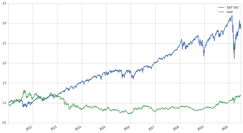
It's evident that the returns of gold are unspectacular, to say the least. It doesn't seem to consistently lose or gain value as much as it meanders around, seemingly uncorrelated to the S&P 500. And indeed, it is almost entirely uncorrelated, with a correlation to the S&P 500 of only 1% over this time period. Is it even worth including in our portfolio? And if it is, how would we determine the allocation size?
Monte-Carlo
To clarify, we're trying to determine the weights for the S&P 500 and gold parts of our portfolio, taking on no leverage:
\[|x_a| + |x_b| = 1\]And maximizing the risk-adjusted return. For every unit of risk we take, we would like to maximize the amount of return we receive. We'll first start off by doing the most straightforward thing, and randomly choosing different weights for our two asset portfolio and then graphing them:
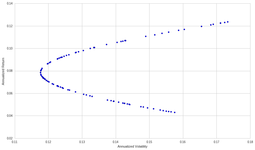
This hyperbola formed is called the Markowitz Bullet, after Harry Markowitz, winner of the Nobel Prize for Economics for his work on Modern Portfolio Theory. The portfolio with the best return vs volatility profile is called the frontier or efficient portfolio. There exists only one such portfolio and it is the portfolio every rational investor should prefer, ignoring borrowings costs and volatility drag (for more information about volatility drag, check out my other post here, or the beginning of my three part series here).
While it's relatively easy to find what would have been the frontier portfolio looking backwards, it is much more difficult to estimate the frontier portfolio over some future time period. We can forecast and then reduce future volatility with modest accuracy, but forecasting expected return is a notoriously difficult problem. So difficult, in fact, that few quantitative investors even try, instead resigning themselves to solely minimize volatility. Likewise, we'll resign ourselves to the same fate.
In the general case of a many asset portfolio, no closed form solution can be found for the minimization of volatility, we must instead use an optimizer or do a Monte-Carlo simulation; but in the two asset case, we can find a symbolic solution. So that's what we'll do next!
Symbolic Solution
Recall that our portfolio return is going to be a function of our two assets and their weights:
\[P = x_a X_a+ x_b X_b\]Likewise, our expected portfolio mean would look like:
\[\begin{align} E[P] &= \mu_P\\ &= x_a E[X_a] + x_b E[X_b]\\ &= x_a \mu_a + x_b \mu_b\\ \end{align}\]And the equation for variance:
\[\text{Var}[X] = \sigma^2 = E[(X-\mu)^2]\]Covariance is similar, except instead of squaring, we multiply each variable after demeaning:
\[\text{Cov}[X,Y] = E[(X-\mu_X)(Y-\mu_Y)]\]Now we just need to derive the portfolio variance:
\[\text{Var}[P] = \text{Var}[x_aX_a + x_b X_b]\]First we substitute for variance and rearrange:
\[\begin{align} \text{Var}[x_aX_a + x_b X_b] =& E[(x_aX_a + x_b X_b - E[x_a X_a + x_b X_b])^2]\\ =& E[(x_a X_a - E[x_a X_a] + x_b X_b - E[x_b X_b])^2] \end{align}\]Now we can pull the constants out of the expectations, substitute, and expand:
\[\begin{align} \text{Var}[x_a X_a + x_b X_b] =& E[(x_a (X_a - \mu_a) + x_b (X_b - \mu_b))^2] \\ =& E[x_a^2(X_a - \mu_a)^2 + x_b^2(X_b - \mu_b)^2 + 2 x_a x_b (X_a - \mu_a)(X_b - \mu_b)] \end{align}\]Finally, we break up the expectations, and replace:
\[\begin{align} \text{Var}[x_a X_a + x_b X_b] =& x^2_a E[(X_a - \mu_a)^2] + x^2_b E[X_b - \mu_b] + 2x_a x_b E[(X_a-\mu_a)(X_b-\mu_b)]\\ =& x^2_a \sigma_a^2 + x^2_b \sigma_b^2 + 2 x_a x_b \text{Cov}[X_a,X_b]\\ =& x^2_a \sigma_a^2 + x^2_b \sigma_b^2 + 2 x_a x_b \rho_{ab} \sigma_a \sigma_b \end{align}\]Where $\rho_{ab}$ is the correlation between $X_a$ and $X_b$:
\[\rho_{ab} = \frac{\text{Cov}[X_a,X_b]}{\sigma_a\sigma_b}\]Now that we have an equation for variance in terms of the weights, mean, volatility, and correlation between the two assets, we can formulate our objective:
\[\min\left( \text{Var}[x_aX_a + x_b X_b]\right)\]Where:
\[x_a + x_b = 1\]We perform the substitution $x_b = 1 - x_a$ and then take the derivative with respect to $x_a$:
\[\frac{\mathrm{d} \sigma_P}{\mathrm{d}x_a}=2 \, \rho_{\mathit{ab}} \sigma_{a} \sigma_{b} - 2 \, \sigma_{b}^{2} - 2 \, {\left(2 \, \rho_{\mathit{ab}} \sigma_{a} \sigma_{b} - \sigma_{a}^{2} - \sigma_{b}^{2}\right)} x_{a}\]Now we set to 0 and solve for $x_a$:
\[x_{a} = \frac{\rho_{\mathit{ab}} \sigma_{a} \sigma_{b} - \sigma_{b}^{2}}{2 \, \rho_{\mathit{ab}} \sigma_{a} \sigma_{b} - \sigma_{a}^{2} - \sigma_{b}^{2}}\]And $x_b$:
\[x_b = 1 - x_a\]Note that sometimes this equation will give us values for $x_a$ and $x_b$ that imply leverage, i.e:
\[|x_a| + |x_b| > 1\]But we can always rescale them by dividing each one by $|x_a| + |x_b|$. In the next section, we'll put this formula to work.
Portfolio Weights
We're going to use a one year or 252 day rolling window to generate the weights. Everyday, we slide our window over one and generate the new weights for that day. Below is the generated graph:
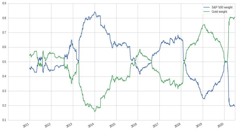
Well that's interesting, the weights change considerably over time. In a real portfolio, not only would we be using an optimizer and a multitude of risk factors to determine the weights, but we would also have constraints on position size, turnover, and the magnitude of deviation from the "ideal" portfolio, and etc. But even in this simple and contrived example, we see that our formula is doing its job: as the volatility of the S&P 500 increases, like at the end of 2018 and during Coronavirus, we start cutting back our equity exposure.
Let's now look at the returns of our portfolio compared to both gold and the S&P 500:
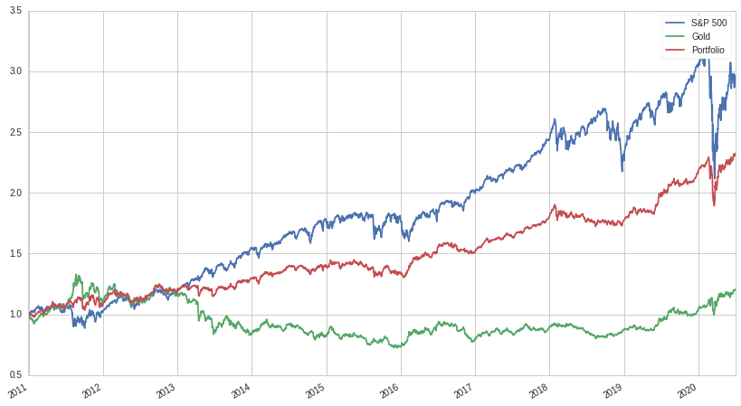
A lot of gains from the market are given up, as we might have expected, but the return stream becomes a lot less volatile. Just looking at a graph of cumulative returns isn't super informative, so here's a table of various metrics:
| Metric | Gold | S&P 500 | Portfolio |
|---|---|---|---|
| Ann. Vol | 15.8% | 17.4% | 10.8% |
| Ann. Ret | 4.3% | 12.4% | 8.4% |
| Beta | 0.01 | 1 | 0.41 |
| Ann. Sharpe | 0.27 | 0.71 | 0.77 |
Wow! Our volatility is lower than either gold or the S&P 500 alone, our beta has been cut more than in half compared to the S&P 500, and our Sharpe ratio is even higher than both! Even with mixing in an asset that had poor returns and high volatility, we've managed to construct a portfolio that, on a risk-adjusted basis, is superior to the S&P 500. And, if we so desired, could be levered up in order to beat the return of the S&P 500, while maintaining comparatively low volatility.
Conclusion
Even with a bad Sharpe ratio and less than stellar returns, gold enhanced our pure equity portfolio. The same also can be said about other, more popular, alternative investments. Hedge funds specifically are often derided for their low returns and frequent meltdowns (such as Long-Term Capital Management); but like with gold, looks can be deceiving. Returns and volatility aren't the whole story. When designing a portfolio, each individual investment is irrelevant, and instead the return stream of the portfolio as a whole is what matters. Considered in isolation, a lot of alternative investments look sub-optimal and irrational. It is only when you zoom out and think about the needs of the investor (their existing allocations, investment goals, monetary needs, etc) does everything come into perspective. When it comes to investing, the whole is certainly greater than the sum of its parts!
I hope you liked the post and if you did, let me know! You can also check out the notebook, developed on Quantopian, here. Possible things you could mess around with are the start and end dates and the two assets to construct a portfolio from.