Just like how there's more than one way to skin a cat, there's more than one way to construct a portfolio. The first systematic method of construction was Modern Portfolio Theory, put forth by Harry Markowitz. MPT's approach is simple: choose weights for each asset that maximize the amount of return received for the amount of risk or volatility taken. However, trying to maximize the risk-adjusted return of a portfolio leads to very unstable allocations, as ex-ante estimates of return are notoriously difficult and previous return isn't a good predictor of future performance.
Another approach that came later is the minimum variance approach which concerns itself with solely minimizing volatility, irrespective of return. While this method might converge on sub-optimal portfolios according to MPT, they tend to be a lot more stable as volatility is easier to forecast than returns. Minimum variance optimization too suffers from some problems: without any constraints, the minimum variance portfolio often heavily weights only a few different assets, suggesting minimal allocations in the rest. For example, given two assets, a stock and a bond, the minimum variance method would almost always return a portfolio in which the bond was allocated the vast majority of the capital. Even if it produced reasonable results, the results are highly unstable: the change in portfolio weights year to year or even month to month can be massive.
For more background on both MPT and minimum variance optimization, check out one of my previous posts: The Value of Alternative Investments. In the mid-90s, a third approach was discovered by the hedge fund Bridgewater, founded by Ray Dalio, that tries remedy some of the problems with both of the aforementioned portfolio construction methods: risk parity.
Math of Risk Parity
Risk parity is a conceptually simple approach to portfolio construction in which we try and construct a portfolio in which each asset contributes a commensurate level of risk to the portfolio. In contrast to a traditional 60/40 portfolio in which the equity component is contributing almost all of the risk, risk parity tries to equalize the risk between each asset. In the two asset case of equities and bonds, the risk parity approach would spit out a set of weights so that each asset contributes equally to the volatility of the overall portfolio. To do this, it would most likely heavily weight the bond compared to the equity. After the weights are determined, the portfolio would be leveraged up in order to match a investor defined volatility budget. With this approach, we often end up with a better risk-adjusted return than a 60/40 portfolio and also get the benefits on diversification, unlike with a minimum variance portfolio.
We're going to use the example of a two asset portfolio with allocation weights $x_a$ and $x_b$ and standard deviations $\sigma_a$ and $\sigma_b$. To keep things explicit, we're going to eschew matrix notation. As we showed in the blog post linked above, the variance of the entire portfolio is:
\[\sigma_P = x_a^2\sigma_a^2 + x_b^2\sigma_b^2 + 2 x_a x_b \sigma_a \sigma_b \rho\]Where $\rho$ is the standard correlation between $x_a$ and $x_b$. So now we want to divide up the risk so that they equal each other. But how do we do that?
To start off, we can use Euler's homogeneous function theorem to help. Euler's theorem states that if a function is homogeneous, i.e:
\[f(tx, ty) = t^n f(x, y)\]Then:
\[n t^{n-1} f(x, y)= x \frac{\partial f}{\partial (x\,t)} + y\frac{\partial f}{\partial (y\,t)}\]In the case of $t=1$:
\[n f(x, y) =x\frac{\partial f}{\partial x} + y\frac{\partial f}{\partial y}\]Well, it turns out that our equation for $\sigma_P(x_a, x_b)$ is homogeneous. By using Euler's theorem, we can figure out how to split up the risk for each asset. First let's calculate the partial derivative with respect to each variable:
\[\frac{\partial \sigma_P}{\partial x_a} = 2(\rho\sigma_a\sigma_b x_b + \sigma_a^2x_a)\] \[\frac{\partial \sigma_P}{\partial x_b}= 2(\rho \sigma_{a} \sigma_{b} x_{a} +\sigma_{b}^{2} x_{b})\] \[n \sigma_P = 2x_a(\rho\sigma_a\sigma_b x_b + \sigma_a^2x_a) + 2x_b(\rho \sigma_{a} \sigma_{b} x_{a} +\sigma_{b}^{2} x_{b})\]Simplifying and solving for $n$ we get:
\[n = \frac{2x_a(\rho\sigma_a\sigma_b x_b + \sigma_a^2x_a) + 2x_b(\rho \sigma_{a} \sigma_{b} x_{a} +\sigma_{b}^{2} x_{b})}{\sigma_P} = 2\]We want each component to be equal:
\[x_a \frac{\partial \sigma_P}{\partial x_a}=x_b \frac{\partial \sigma_P}{\partial x_b}\] \[\rho\sigma_{a}\sigma_{b}x_{a}x_{b}+\sigma_{a}^{2}x_{a}^{2} =\rho \sigma_{a} \sigma_{b} x_{a} x_{b} + \sigma_{b}^{2} x_{b}^{2}\]Assuming:
\[x_a + x_b = 1\]We substitute $x_b = x_a - 1$ and then solve for $x_a$. Discarding the negative solution, we get:
\[x_a = \frac{\sigma_b}{\sigma_a + \sigma_b}\]And solving for $x_b$:
\[x_b = \frac{\sigma_a}{\sigma_a+\sigma_b}\]Note that the solution does not depend on the correlation $\rho$, which some might find counter-intuitive. While we showed that there exists a closed form solution for the case of two assets, a numerical solution is required when $n>2$.
Risk Parity in Practice
We're going to construct a risk-parity portfolio from two assets: SPY (S&P 500), and LQD, which is an investment grade bonds ETF. Our weights will be calculated as described above, using a 252-day rolling window for the volatility calculations. Below is a graph of the weights over time:
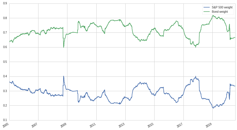
As expected, bonds make up the majority of the portfolio in order to match the risk of the equity component. Let's look at the cumulative returns of our risk parity portfolio compared to a traditional 60/40 portfolio:
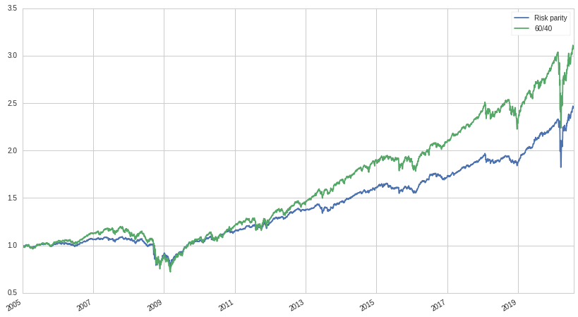
Due to the majority of our risk parity portfolio being bonds, the portfolio underperforms a classic 60/40 portfolio that takes on significantly more equity risk. Having a relatively low natural return is expected of a risk parity portfolio, which is why leveraged is applied after portfolio construction. But what leverage ratio to use? In order to have an apples-to-apples comparison between a risk parity portfolio and a 60/40 one, we will leverage up in order to try and match the volatility of a 60/40 portfolio:
\[l = \frac{\sigma_{60/40}}{\sigma_{RP}}\]For each $\sigma$, we use a 252-day rolling window. We calculate the leverage ratio needed on each day and leverage up accordingly. Ideally, this will ensure that the amount of risk taken by the risk parity portfolio is always inline with the amount of risk a 60/40 portfolio is taking. Let's look at a graph of our leveraged risk parity portfolio, a classic 60/40 portfolio, and the leverage ratio:
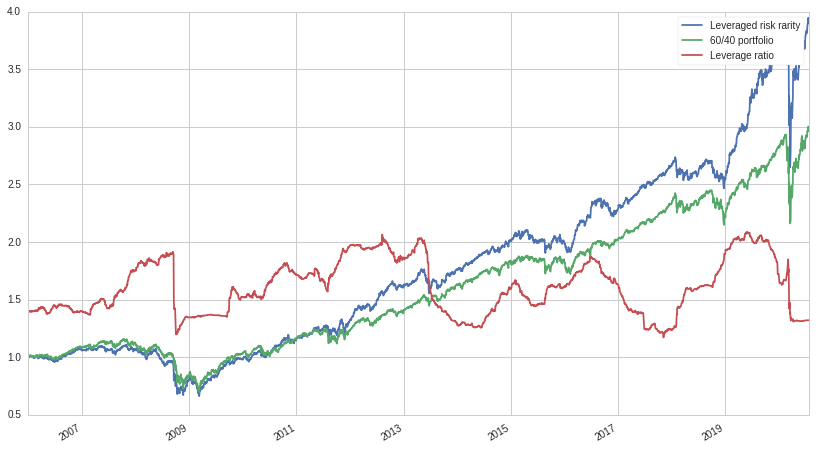
Not bad! The amount of leverage taken is reasonable and the performance of the risk parity portfolio looks pretty good. Let's look at a table of metrics:
| Metric | Risk Parity | 60/40 |
|---|---|---|
| Beta | 0.51 | 0.68 |
| Ann. Ret | 9.9% | 7.8% |
| Ann. Vol | 12.8% | 12.8% |
| Ann. Sharpe | 0.77 | 0.6 |
Our simple dynamic leverage strategy works very well, with the volatility of the two portfolios being identical. But even with the same volatility, the risk parity portfolio significantly outperforms while also having less beta exposure and a better Sharpe ratio as well. Another plus is that the amount of leverage taken is very reasonable, and well within the ability of even retail investors to obtain.
Conclusion
Risk parity is an exciting and effective technique that is a viable alternative to minimum variance portfolios as well as fixed weight portfolios such as 60/40. While risk parity portfolios might not reduce volatility as much as minimum variance portfolios, they tend to be more stable over time, incur less turnover, and provide greater diversification. Compared to a 60/40 portfolio, they are usually superior unless the borrowing costs are too high. This interest rate exposure represents a distinct risk for risk parity strategies; a risk investors should be cognizant of.
Thanks for reading and hope you liked this post! You can check out the Quantopian notebook here. Feel free to change the time periods and assets used to construct the portfolio.