In part one of this three part series, we will explore the concept of levered ETFs, common misconceptions, the effect of volatility on the returns of a portfolio, and the compounded returns of the S&P 500 utilizing different leverage ratios. We will also touch on the basic mathematical underpinnings of volatility drag and ideal leverage ratio.
In part two, we will look into different ways to forecast future market regimes and their associated optimal leverage ratios.
In part three, we will construct a fully automated ETF that seeks to obtain variable leveraged exposure to the S&P 500 conditioned on the future forecasted market return and volatility regime.
Background
The recent ascent of ETFs as one of the most popular trading vehicles for both retail and institutional investors has dramatically affected the business of all funds seeking retail flows, and even many who do not. ETFs and ETNs serve as wrappers for a diverse array of strategies that run the gamut from simple and transparent to complex and proprietary. ETFs (and ETNs though for brevity's sake we will just refer to all securities employing this legal structure as "ETFs") can be placed on a two dimensional spectrum: simple to complex on one axis, and transparent to proprietary on another. These products are united by several distinguishing features: placement on public equity markets with tickers alongside equities and a pricing mechanism that, also much like equities, utilizes arbitrage and a bid-ask mechanism that is used by market makers to provide liquidity. ETF shares are created and destroyed in blocks as needed in order ensure that the value of the wrapper is inline with the value of the underlying securities or strategy that the ETF conceptually represents.
By far the most popular type of ETF in terms of total asset value and flows are ETFs that provide exposure to popular indices such as the S&P 500, the Russell 2000, and many others. These ETFs simply aim to match the relative daily returns of their respective index and occupy the bottom left spot on the aforementioned two dimensional spectrum. A closely related (albeit far less popular) type of product that occupies the bottom middle is the leveraged ETF. A leveraged ETF seeks to obtain a daily exposure on an underlying index scaled by a constant $l$; which, at this time, is somewhere between -3 and 3 for products currently on the market. If $l$ is less than zero, the ETF provides short exposure to the index and are often called "bear" ETFs; conversely, if $l$ is greater than zero, the ETF provides long exposure to the index, commonly referred to as "bull" ETFs. These securities are usually implemented by means of a rolling futures strategy. By rebalancing everyday, the ETFs eliminate the risk of ruin (in this case, losing more money than the fund's total value) and obviate the need for margin payments.
The Popular Argument Against Leverage
At face value, a retail investor might assume that if the S&P 500 returned 10% in a given year, a 3x leveraged ETF would return 30%. Fortunately or unfortunately depending on your perspective, this is not the case as the ETF seeks to maintain a 3x multiple on the daily return of the S&P 500 instead of the annualized return. As touched on in the previous section, by rebalancing daily the ETF can easily handle the inflows and outflows of the fund while also eliminating the need for capital to be held in margin. This strategy also greatly reduces the risk of ruin, as the S&P 500 would need to lose at least 1/3 of its total value in a single day for the fund to be wiped out. Though certainly imaginable, this event is unlikely as the biggest single day loss in the history of the S&P 500 was Black Monday in 1987, in which around 20% of value evaporated from the S&P 500 in a single day.
The common wisdom about leveraged ETFs is that they don't so much fill a roll as an investment vehicle, but merely as a day-trading instrument that allows a trader to easily obtain short-term tactical Beta exposure to the market in an efficient and simple fashion. In numerous articles scattered across the internet, the author always drives home the point again and again that leveraged ETFs are ill-suited to long-term buy-and-hold investing and should only be purchased by those who are savvy enough to lay on short-term trades. Instead of cementing this advice on a solid mathematical foundation, the author usually cherry picks some example time window for the S&P 500 of around two months where the market is mostly sideways and volatility is high. He then usually remarks on the prescient insight that the levered fund made less or even lost money whilst the regular fund came out ahead. The conclusion to be drawn from this I suppose is that levered funds are deceptive, don't actually multiply your returns by the amount claimed, and are a bad investment. In the next section, we will discuss the mathematical foundation of this claim and reason about its validity.
A Little Bit of Math
We can see the immediate effect of volatility from a simple example. What happens to a $100 portfolio that gains and then loses 10% of its value versus a portfolio that gains and then losses 50%?
\[\$100(1.10)(0.90) = \$99\] \[\$100(1.50)(0.50) = \$75\]As we can see, the difference between the arithmetic mean (which for both examples is 1) and the geometric mean (appropriate for compounded returns) can be quite significant. In order to calculate the effect that volatility has on a portfolio we can use the volatility drag formula:
\[r_a = r_p - \frac{\sigma^2_p}{2}\]Where $\sigma_p$ is the standard deviation of the portfolio, $r_p$ the return of the portfolio and $r_a$ the actualized return of the portfolio after deducting for volatility.
It's important to understand that the value of the volatility drag equation is when we are changing the volatility of a known return stream. If we are using past realized returns to forecast future returns, the volatility equation isn't necessary or applicable, since the past returns are already reflective of the post-drag return. The volatility drag equation becomes useful when we are asking ourselves about the returns of a levered portfolio in terms of the unlevered returns and volatility. Alternatively, the equation also comes in handy if we would like to answer questions such as: If we reduced the volatility our of current portfolio by 25%, how would that affect the mean return?
We need to rewrite the volatility drag equation in terms of leverage. Assuming normality, we see that rescaling a normal distribution by a constant affects the mean linearly and the variance non-linearly (thus affecting the standard deviation linearly):
\[Y = lX \sim N(l\mu, l^2\sigma^2)\]In other words, a 2x levered portfolio with a mean return of 5% and a volatility of 5% is the same as an unlevered fund with a mean return of 10% and a volatility of 10%. As such we can rewrite $r_p$ in terms of $r_b$ (the base unlevered return of the portfolio) and the leverage amount ($l$):
\[r_p = r_bl\]As well as $\sigma_p$ in terms of $\sigma_b$ and $l$:
\[\sigma_p = \sigma_bl\]Substituting into our drag equation:
\[r_a = r_bl - \frac{\sigma_b^2}{2}l^2\]In order to find the maximum leverage that will result in the greatest mean return, we then take the derivative in terms of the leverage ratio and set to zero and solve:
\[\frac{\text{d}(r_a)}{\text{d}l} = r_b - \sigma^2_bl = 0\] \[l = \frac{r_b}{\sigma^2_b}\]Also, our adjusted Sharpe ratio is:
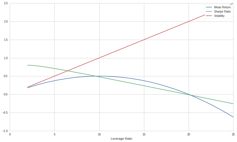
\[S_a = \frac{r_b}{\sigma_b} - \frac{\sigma_b}{2}l - \frac{r_f}{\sigma_bl}\]Below is a graph of the adjusted Sharpe ratio, volatility and mean return of a portfolio given $r_b= \sigma_b=10\%$. We can see that the returns form a concave quadratic, the Sharpe ratio a negative linear function, and the volatility a positive linear function. Note that in this graph we are using log returns:
An interesting and important property of volatility drag is that even if two portfolios look the same given a specific leverage ratio, after the drag calculation, they often end up quite different. Below is a table of different example portfolios and leverage ratios that illustrate this point:
| Portfolio | Return | Volatility | Leverage | Pre-drag Return | Post-drag Return |
|---|---|---|---|---|---|
| A | 1% | 1% | 5 | 5.025% | 4.9% |
| B | 5% | 5% | 1 | 5.125% | 5% |
| C | 10% | 10% | 0.5 | 5.25% | 5.125% |
We found the pre-drag return values by first calculating the natural unlevered return given no volatility and then scaling it by the leverage ratio:
\[r_{pre} = l \left( r_p + \frac{\sigma^2_p}{2} \right)\]To calculate the post-drag return values in the table, we use the regular volatility drag equation but use the pre-drag return and levered volatility as inputs:
\[r_{post} = r_{pre} - \frac{(\sigma_pl)^2}{2}\]As we can see, if we are choosing between multiple portfolios with the same Sharpe ratio, we should always prefer the portfolio that has the highest natural return. For portfolio A, we pay a significant cost in volatility. Portfolio B pays no cost, as the historical return has already taken into account the realized volatility. Portfolio C actually outperforms the natural portfolio B, since we get some volatility "lift" from deleveraging. The takeaway is that the Sharpe ratio is not a sufficient distillation of a portfolio or strategy due to the concave quadratic nature of volatility drag. Instead, we need to also look at the unlevered mean return of the strategy, as well as the Sharpe, in order to determine the actual quality of the strategy. In some cases, it would actually be preferable to choose a strategy with a lower Sharpe ratio than one with a higher ratio if the mean unlevered return of the former is sufficiently greater than the latter.
Historical S&P 500 Returns and Leverage
While the leverage ratio formula is correct if we are sampling from a normal distribution, market returns often exhibit excess kurtosis and skew, resulting in the decreased accuracy of our formula. The greater the skew or kurtosis, the less accurate the model becomes. In periods of positive skew, the model underestimates the magnitude of mean return, while in negative skew, the model overestimates the mean return. Below is a density plot of returns between 2018-01-01 and 2019-09-01:
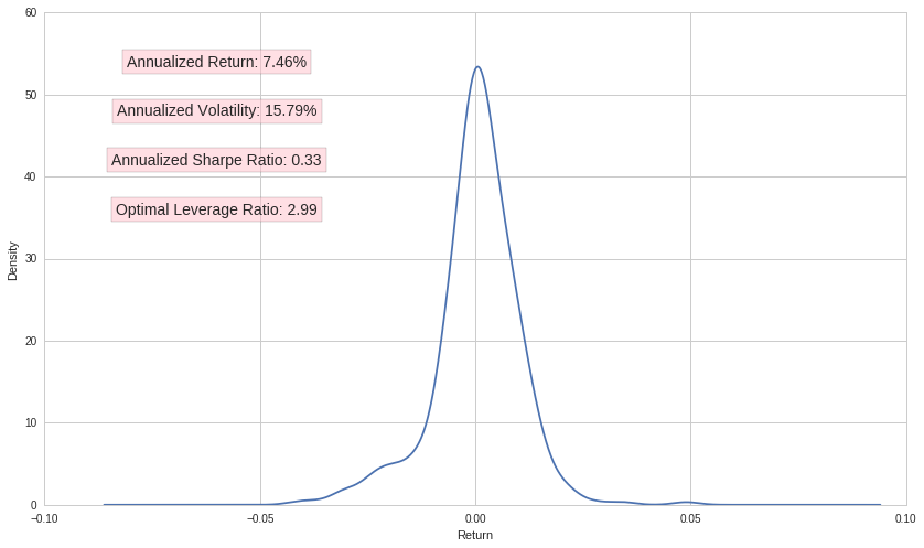
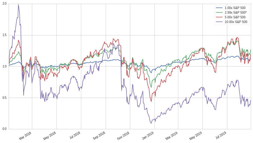
For this periods volatility and returns, the model equation suggests a leverage ratio of approximately 3 in order to maximize returns. Looking at the cumulative return streams of several different leverage ratios, we see that despite the non-normality of the data, the prediction is solid:
Unfortunately, the use of variable leverage conditioned on volatility and returns does not yet constitute a viable trading strategy: during actual trading, future volatility and return information is not available. Without a model to estimate the future returns and volatility of the market, we will be unable to effectively calculate the optimal leverage ratio for our portfolio. There are several remediations of varying complexity and accuracy that we could use to work around this problem. The most basic model we could employ would be one that uses a trailing window of returns and volatility in order to predict the future returns and volatility. Other options would be to use statistical time series models such as ARIMA (Auto-Regressive Integrated Moving Average) in order to forecast returns and GARCH (Generalized Auto-Regressive Conditional Heteroskedasticity) to predict volatility. Other approaches might include looking at the VIX (Volatility Index) or even constructing RNNs (Recurrent Neural Networks) to help forecast an ideal leverage ratio.
Conclusion
While the Sharpe ratio of a levered index ETF will indeed get worse as leverage is applied, the use of leverage and the associated volatility drag does not constitute a separate and distinct issue aside from volatility alone. For all investors, return and volatility are intimately related through a portfolio's Sharpe ratio. Ultimately though, investors cannot eat risk-adjusted returns and must instead try to maximize the Sharpe ratio of their respective portfolios in order to always assume the greatest amount of risk in line with their investment objectives. For most investors, alpha generation through security selection and trading is a lofty and unattainable strategy. Instead of chasing elusive alpha, these investors adjust the lever of risk through the management of asset class and factor exposures. When market volatility is higher than personally tolerable, investors cycle into lower volatility investments such as value stocks, bonds, and metals. When volatility and the associated risk-premium is too low, investors rotate into growth stocks, emerging markets, and real estate.
In this post we touched on a different and arguably simpler way to manage volatility and risk-premiums: through the conditional application of leverage. In part two of this three part series, we will look at ways to forecast the ideal leverage ratio as a function of three parameters: future returns, volatility, and personal risk limits.
Thanks for reading, I hope you enjoyed this piece! If you want to play around with the Quantopian notebook, click here! Possible things to change would be the start and end dates, reference leverage ratios, and the ticker to analyze.