In this post, we will look into the relationship between diversification, risk, and leverage: first covering the history of diversification and risk and then expounding upon the mathematical link between leverage and diversification. Much of the material in this post is related to another post of mine which you can view here: ETFs, Volatility and Leverage: Towards a New Leveraged ETF Part 1.
While this article doesn't constitute the next post in the series (stay tuned!), it covers some important ideas that I feel to have tangency to the ideas put forth in the earlier post. So without further ado, let's jump into the origins of diversification!
Background
Diversification, the strategy of investing in multiple unique return streams or investments simultaneously, has been a portfolio construction technique used to mitigate risk for thousands of years. The concept is mentioned in several ancient religious texts, including the Bible and Talmud, and came to prominence under the Roman Empire: investors would form investment partnerships for particularly risky business endeavors, such as financing the voyages of merchant vessels. While the original purpose of these partnerships was to provide access to lucrative investment vehicles for investors lacking sufficient capital to fund such a voyage alone, they quickly became popular as risk-pooling strategies; for even the richest Romans would often buy shares of many different voyages in order to diversify the significant risk of any single voyage.
The modern concept of diversification was popularized by Harry Markowitz in the 1950s through his concept of a Markowitz-efficient portfolio (MEP) and Modern Portfolio Theory (MPT). A MEP is a portfolio that lowers the portfolio's volatility through diversification for a given level of expected return. Or alternatively, the portfolio with the lowest volatility possible (achieved primarily through diversification) that still satisfies a minimum level of expected return. MPT and MEP were the first formalizations of diversification put forth, creating a framework for viewing the essence of a portfolio through its return and volatility. of a portfolio through the return and volatility of the portfolio. Using the example of a discretionary equity investor, the MEP would consist of as many stocks as the investor could find or research that would pass his investment criteria. Once the investor started adding less desirable stocks (stocks with a lower expected return) that culminate in a portfolio with lower return than the desired or expected return, he no longer would hold a MEP.
More generally, Markowitz in MPT introduced the concept of the Capital Market Line (CML):
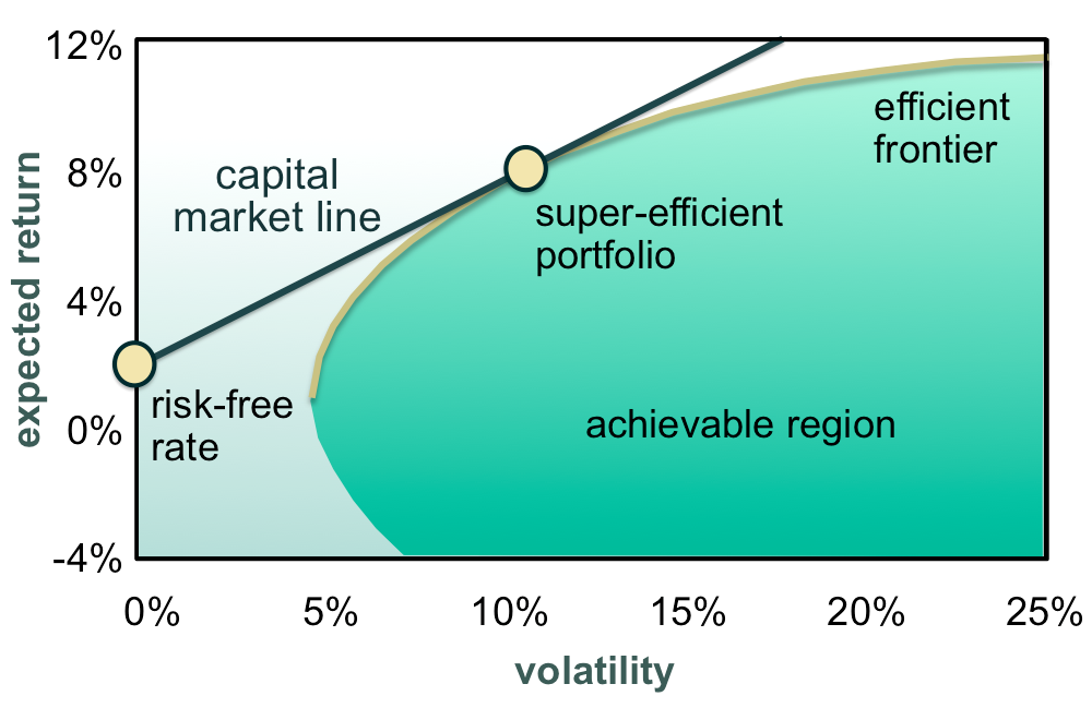
The efficient frontier is any portfolio that possesses the highest risk-adjusted return: the portfolio that had the highest expected return as a function of volatility. While any portfolio on the efficient frontier is superior to any risky portfolio in the achievable region, by using the risk-free rate to find the super-efficient portfolio, also called the tangency or market portfolio, we can create a portfolio that is a linear combination of risk-free assets and risky assets. By either going long or short the risk-free rate (lending or borrowing), we can achieve any level of return as a function of volatility or vice versa. While this is not strictly true for a compounding portfolio due to volatility drag (see my aforementioned post), the intuition behind it is powerful. We can then see risk as a multiple on the volatility of the super-efficient portfolio.
Later with the advent of the Capital Asset Pricing Model (CAPM) and multi-factors, the concept of risk was partitioned into two primary categories: systematic and specific risk. Unlike specific risk which can be diversified away through the holding of a MEP or similar portfolio, systematic risk cannot be easily diversified as it represents the latent factors in which all assets have some exposure to. In the original formulation of CAPM, specific risk was assumed to be zero and not included in the equation:
\[r_i - r_f = r_f + \beta_i (r_m - r_f)\]Where $\beta_i$ is $\frac{\text{Cov}(r_m,r_i)}{\text{Var}(r_m)}$, $r_f$ is the risk free rate, $r_i$ is the expected return of the asset $i$, and $r_m$ the expected return of the market. The introduction of CAPM by William Sharpe and others was the next pivotal step after MPT in quantifying risk and transformation finance into a legitimate scientific discipline. In CAPM, a portfolio's risk is defined as some multiple of the market's risk, generally assumed to be the volatility of the market. This important idea is best visualized by the Security Market Line (SML):
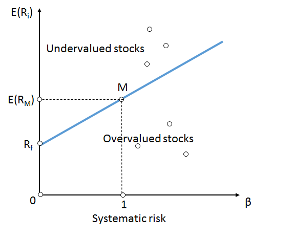
Though under the CAPM model, investors may choose where on the line best fulfills their investment goals ($\beta$) through portfolio construction, they are not easily able to diversify away their market risk since, by definition, their $\beta$ will converge to 1 as more and more assets are added to the portfolio; nor can investors capture excess returns relative to the market risk, as per the Efficient Market Hypothesis both overvalued and undervalued stocks mispricings will be arbitraged away. In it's essence, CAPM posits that investors are compensated in the exact same proportion to the market risk assumed, revealing an interesting property of specific risk: since specific risk can easily be hedged away through the construction of a MEP, investors are only compensated for systematic or market risk assumed, not specific risk. A consequence of this is that investors are more likely to judge an asset by its systematic risk versus its specific risk: an investment with low sensitivity to the market but high specific risk may be judged to have much less risk than a naive observer might expect.
In the next section, we look at the mathematics of diversification of random variables.
Portfolio Variance and Diversification
An interesting proprety of diversification is that mathematically speaking, with every new security we add to our portfolio, the volatility of the portfolio monotonically decreases as long as two conditions are met: the correlation of the new asset to any other asset is less than 1, and that the sum of portfolio weights never increases. Let's define a portfolio $P$ that is a linear combination of two variables (assets):
\[P = x_A X_A + x_B X_B\]where $x_A$ and $x_B$ are the proportion or weights of the assets in the portfolio. While the returns of the portfolio are a linear combination of the two return streams of the assets, the variance is:
\[\sigma_P^2 = x_A^2 \text{Cov}(r_A,r_A) + x_B^2\text{Cov}(r_B,r_B) + 2x_Ax_B\text{Cov}(r_A,r_B)\]Though it may not be immediately obvious, the variance of the portfolio will always be lower the more assets we add, as long as the aforementioned conditions are met. With three or more assets, the equation starts to become too unwieldy so instead, we often represent the variance of a portfolio using matrices. Using the same example of two assets, $X_A$ and $X_B$, we first define the covariance matrix:
\[\textbf{P}=\begin{bmatrix} \text{Cov}(r_A,r_A) & \text{Cov}(r_A,r_B) \\ \text{Cov}(r_B,r_A) & \text{Cov}(r_B,r_B) \end{bmatrix}\]Next we define our vector weights or proportions:
\[\textbf{x}= \begin{bmatrix} x_A \\ x_B \end{bmatrix}\]Now we can define our variance in terms of the covariance matrix and the vector weights:
\[\sigma_P^2 = \mathbf{x}^T\mathbf{Px}\]This is often called the quad or quadratic form of $\mathbf{x}$ and $\mathbf{P}$.
In the special case where:
\[x_A + x_B = 1\] \[x = x_A = x_B\] \[\sigma = \sigma_A = \sigma_B\] \[\rho_{AB} = 0\]Then:
\[\textbf{x}= \begin{bmatrix} x \\ x \end{bmatrix}\] \[\textbf{P}=\begin{bmatrix} \sigma^2 & 0 \\ 0 & \sigma^2 \end{bmatrix}\] \[\sigma_P^2 = \mathbf{x}^T\mathbf{Px} = \frac{\sigma^2}{2}\] \[\sigma_P = \frac{\sigma}{\sqrt{2}}\]In the general case of $n$ assets:
\[\sigma_n = \frac{\sigma}{\sqrt{n}}\]The graph below visualizes the portfolio volatility as a function of assets each with a standard deviation of 10%:
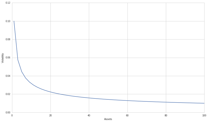
This graph makes it very clear on why investors are not compensated for bearing specific risk: is is relatively easy to reduce much specific risk by holding a relatively small number of assets in a portfolio. Even though for equities in particular the volatility cannot be reduced as much due to most equities being highly correlated to each other through their common systematic risk factors, as we will see in the next section, we can still get most of the way there with only 20-30 different correlated assets.
In the next section, we will look at some market data and run some simulations in order to better understand the effect of diversification on a theoretical portfolio under real market conditions.
Diversification and Historical S&P 500 Returns
To illustrate how diversification affects volatility and returns in a real market environment, we ran a Monte Carlo simulation that generated 1000 random portfolios that long $n$ number of random stocks, where $n$ is all even numbers between 2 and 100, inclusively. All stocks were chosen from the S&P 500 and the daily portfolio returns were constructed between 2017-01-01 and 2019-01-01. Below is a graph of average annualized volatility and return as a function of assets held:
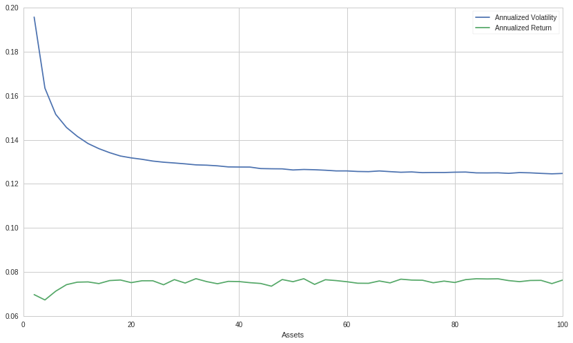
In contrast to the essentially constant annual return as a function of assets, the volatility exhibits a sharp downward trend before stabilizing, reminiscent of the previous graph of perfectly uncorrelated assets all sharing the same volatility. Since we are picking stocks randomly, it is unsurprising that we trend toward the MEP with the same expected level of return regardless of how many assets are in the portfolio. Though not shown on the graph, the average annualized volatility of our portfolio unsurprisingly trends quickly toward the annualized volatility of the S&P 500 during that same period.
Leverage
Despite the prior graph implying that the volatility and return of our portfolio exist orthogonal to one another, in reality for a compounding portfolio, this is not actually the case. The essence of the problem is in the AM-GM Inequality, also called the inequality of arithmetic and geometric means:
\[\frac{1}{n} \sum_{i=1}^{n}x_i \geq \left(\prod_{i=1}^n x_i \right)^{1 \over n}\]This equation implies that the arithmetic average of our returns will only be accurate if and only if the return stays constant. Otherwise, our true geometric returns will always lower than the arithmetic return. Thus, due to the nature of compounding returns and geometric sums, the volatility of our portfolio has a very real negative affect on our long-term returns. This phenomenon is coined volatility drag and increasingly penalizes portfolios with higher and higher volatility:
\[r_a = r_p - \frac{\sigma^2_p}{2}\]Where $\sigma_p$ is the standard deviation of the portfolio, $r_p$ the return of the portfolio and $r_a$ the actualized return of the portfolio after accounting for volatility drag (for a more in-depth dive into volatility drag see the link at the beginning of this post). Volatility drag implies that not only should we aim to reduce volatility for the classically given reasons, but that reducing volatility actually lets us boost our returns, which means that diversification provides even more benefit than we might otherwise think.
Leverage and Diversification
A key result of my linked post is the relationship between volatility, return, and leverage. After a little bit of math we arrived at the conclusion that in order to maximize our return, we should lever up our portfolio as per the following equation:
\[l = \frac{r_b}{\sigma_b^2}\]Some of the readers might notice the similarity between the ideal leverage ratio and the fractional Kelly:
\[f^* = \frac{\mu-r}{\sigma^2}\]Regardless, we can look at the ideal leverage ratio as a function of the number of assets in our portfolio:
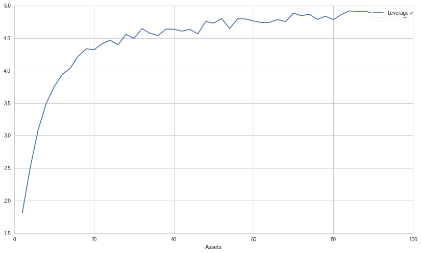
We can see that the optimal leverage for maximizing the geometric growth of our portfolio increases quickly relative to the number of assets in our portfolio but also rapidly stabilizes at a leverage ratio between 4.5 and 5 between 2017-01-01 and 2019-01-01.
It is now evident that diversification can be used in one of two ways: to reduce the uncompensated specific risk of a portfolio, or to increase the amount of risk or leverage we as investors can take in order to maximize the long-term geometric growth rate of our portfolio. In general, we should always aim to maximize our risk while satisfying our risk controls in order to generate the greatest possible return. Diversification allows us to minimize specific risk, in which we are not compensated for, giving us the opportunity to obtain risk for which we are compensated for, namely, systematic risk.
Conclusion
In this post we arrived at a couple important conclusions. We can easily reduce our volatility through diversification, even when picking random assets for our portfolio. Not only does this reduce our risk, but it has the potential to boost our returns as well. Taking it a step further, we can actually lever up our portfolio in order to maintain risk parity if we so choose. Thus we can use diversification in one of two ways: to either greatly reduce risk and modestly boost the compounded returns of our portfolio, or to lever up the less risky diversified portfolio in order to maximize the long-term geometric growth. Either way, diversification is a powerful tool in an investor's toolbox and should be exploited to its fullest potential. Furthermore, because diversification reduces volatility drag and boosts our returns, in addition to allowing us to take more leverage, it very well might make sense to diversify past the point of a MEP, as the long-term compounded savings could outweigh the decrease in single-period expected return.
Thanks for reading, I hope this was entertaining and informative! If you want to check out the Quantopian notebook I made for this post, click here! Feel free to experiment with different start and end dates, number of assets, or trials. If you clone the notebook and play with it, you must also put a file called "SP500.csv" in your data directory. Simply copy the data off of Wikipedia or some other source and format it to be a one column CSV file with the header "Ticker".
(1) Check out my deep dive into volatility and leverage: ETFs, Volatility and Leverage: Towards a New Leveraged ETF Part 1. It clarifies some of the concepts in this post and derives the equation for leverage that we used in the previous section.