The beta exposure of a stock is one of the first and most important statistics any investor looks at. Though perhaps simplistic, it distills a myriad of various properties of a stock into a single, easily digestible number. Using beta, it becomes easy to roughly forecast how an investor's portfolio would perform under different market conditions. Maybe out portfolio has a beta of 1.3 and we expect the market to return 11% next year: great, our portfolio should return around 14.3% (1.3*11%). While there's a lot of problems with this simplistic model, in this post, we're going to focus on just one: the beta of a stock changes significantly over time. Consider this graph of Apple's rolling, 252-day beta:
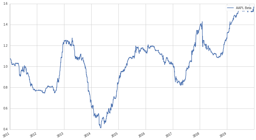
As we can see, the dispersion is quite high, and the rolling beta rarely stays the same for any reasonable period of time. There could be any number of reasons for why the rolling beta changes, such as changes in the drivers of market movements, the evolution of Apple's business model, geographic changes in sales, and etc.
Clearly, some companies are going to have higher beta stability than others. One might imagine that a mature utility company with stable recurring revenue would have greater beta stability than a recently IPO'd tech company who's revenue model and business units are still in flux. So that brings up the question, when constructing a portfolio, which kind of companies would we prefer: the relatively unstable beta company, or the more stable one? In this post, we're going to form and test the hypothesis that, in the long run, a portfolio that consists of stocks with high beta stability generates excess returns.
The Beta Stable Factor
Our goal is to construct a beta neutral long/short portfolio that tries to capture the abnormal return that we hypothesized might be associated with a beta stable portfolio. To do this, we're going use to the Q500US universe provided by Quantopian. This universe consists of the top 500 most liquid (and therefore, probably largest market cap) equities on any given day. We construct our alpha factor as follows:
\[f = \text{Z}[\text{rank}(-|\beta_{21}-\beta_{63}|)]\]Where $\beta_{21}$ is the 21-day (one month) rolling beta, and $\beta_{63}$ the 63-day (three month) rolling beta. We then take the absolute value, negate, rank, and Z-score. This factor gives us a portfolio that goes long stocks that have lower changes in beta and shorts those that have greater changes in beta.
Because we suspect that higher beta stocks tend to have more instability, we will zero out the beta exposure by dynamically adjusting our net long exposure. We use the same method that we did in The Low Beta Anomaly post, so go check it out if you want the details. Backtesting over a 10 year period, 2010-01-01 to 2020-01-01, let's first look at our net long exposure:
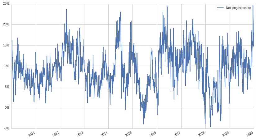
The reason for our net long exposure being positive is that there is some correlation between beta instability and high beta stocks. Beta generally has a right hand skew, so our unadjusted portfolio would have a higher average beta for the short-side than the long-side. Overall, this would result in a portfolio that had significant negative beta exposure, an undesirable property to have in a world where the market usually goes up. By increasing the long-side of our portfolio, we can offset the high beta short-side and maintain beta neutrality. Even so, the net long exposure is relatively small compared to what we observed for our low beta portfolio (again, to compare, check out The Low Beta Anomaly post): around 10% vs 45%, respectively. This is good, because it means we are capturing an independent effect with our beta stability hypothesis, not just another reformulation of the low beta/volatility anomaly.
Now for the good part, the cumulative return over the same time period:
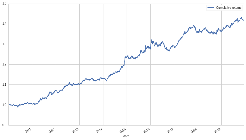
Wow, that looks pretty good for a beta neutral strategy! Let's decompose the returns into quantile:
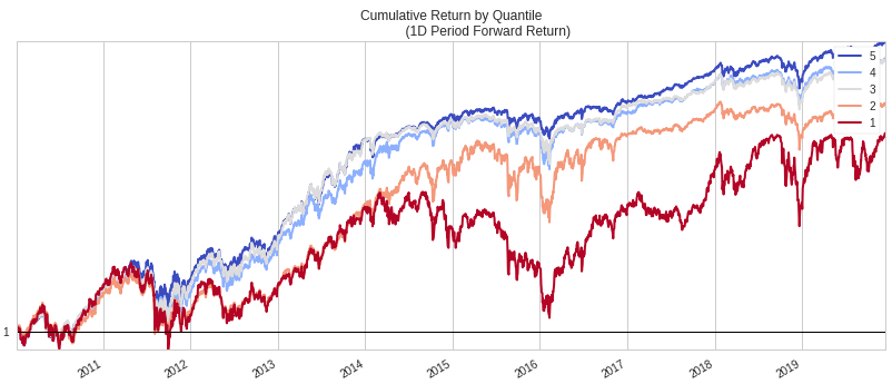
This graph shows the cumulative return by quantile if each quantile was held long (remember that the lower quantiles are held short in our portfolio). The profit from our strategy comes from the difference between the upper quantiles and the lower ones. Let's look at a table of metrics to better understand the strategy:
| Metric | Value |
|---|---|
| Beta | -.018 |
| Ann. Ret | 3.56% |
| Ann. Vol | 2.7% |
| Ann. Sharpe | 1.28 |
Not bad at all! Our beta minimization worked well, the return is pretty significant, and our Sharpe ratio is very respectable, at 1.28.
Even so, in an ideal beta neutral strategy, we would want to be making money off the short-side of the portfolio, not merely hedging our market risk with it: i.e, we would want to see the lower quantiles lose money, not merely make less than the greater quantiles. In the next section, we'll consider a long-only variation of the same beta stable strategy.
Long-only Beta Stable
For the long-only variation, we'll use the same factor as before, but instead of investing in the entire Q500US universe, only invest in the top 100 stocks. This will give us a portfolio with higher allocations to stocks with greater beta stability and one with 100% net long exposure. Using the same time period, consider the quantile graph below:
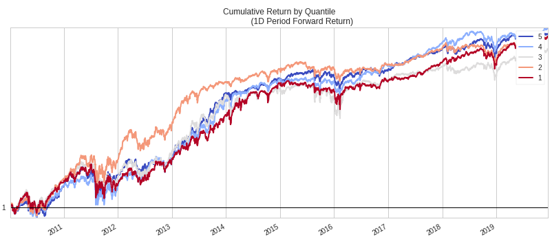
As expected, we only see a small difference of the returns by quantile. This is because we are only investing in the 100 most stable equities, significantly narrowing the gap between the lowest and highest quantile. Still, there is some effect (the first quantile realizes the lowest returns), which bodes well for the robustness of our factor. Now, for the moment of truth, our factor portfolio compared to the S&P 500:
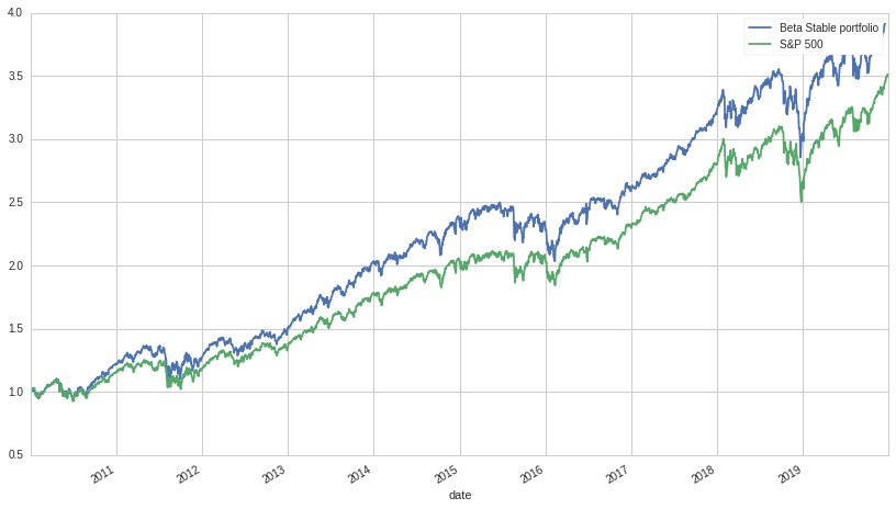
Wow! This is an amazing result: over a 10 year period, our factor portfolio returns a little under a 50% superior return compared to the S&P 500. Here's a table of metrics for comparison:
| Metric | Portfolio | S&P 500 |
|---|---|---|
| Beta | 0.99 | 1.0 |
| Ann. Ret | 14.7% | 13.37% |
| Ann. Vol | 15.5% | 14.6% |
| Ann. Sharpe | 0.94 | 0.91 |
With over a 1% of excess return, a higher Sharpe ratio, and an equivalent beta, the long-only beta stable strategy appears to be a huge success!
Conclusion
Based on the results, perhaps we should consider beta stability a new persistent factor, alongside the classics like low-volatility, value, and size? This is a bold claim of course, and much more research needs to be done; but the preliminary results are very positive, especially for the long-only version. It would be very easy to overlay onto an existing beta exposed portfolio, generating a moderate amount of excess return without taking on any more risk. The beta neutral version also has promise, though ideally it would be combined with other factors (such as maybe value or low-beta) in order to boost the Sharpe ratio and unleveraged return.
Thanks for reading, I hope you enjoyed this post! for the source code, check out the Quantopian notebook here. Feel free to play around with the start and end dates, universe, and anything else. If you have any comments or feedback, contact me at sturm@cryptm.org.