Perhaps more than any other development, finance was ushered into the modern era with the development of the Capital Asset Pricing Model (CAPM) by William Sharpe in the early 60s. Though commonly criticized as too simple and reductionist, the model is still used today as an easy way to determine a stock's exposure to the market:
\[r_i - r_f = r_f + \beta_i (r_m - r_f)\]$\beta_i$ was originally formulated as $\frac{\text{Cov}(r_m,r_i)}{\text{Var}(r_m)}$, but it is more commonly calculated by taking the slope of a linear regression between the asset and the market. $r_m$ is the expected market return, $r_f$ is the expected risk-free rate, and $r_i$ is the expected return of the asset.
Perhaps the model is so popular because the interpretation of $\beta$ is so concrete and easy to understand: a stock's $\beta$ is simply a multiplier on the market's return. Stocks with high betas are more volatile than the market, and those with smaller betas less so. In tumultuous times, investors try and cut their volatility by rotating into low beta stocks; while in bull markets, investors clamor to those with the highest betas.
There's been a problem with CAPM, and indeed, the very concept of beta, for a long time now: it's called the low beta anomaly. Academics noticed that there was systematic discrepancies between high and low beta stocks: it seemed like higher beta stocks were under performing and low beta stocks were outperforming. Consider the Security Market Line (SML):
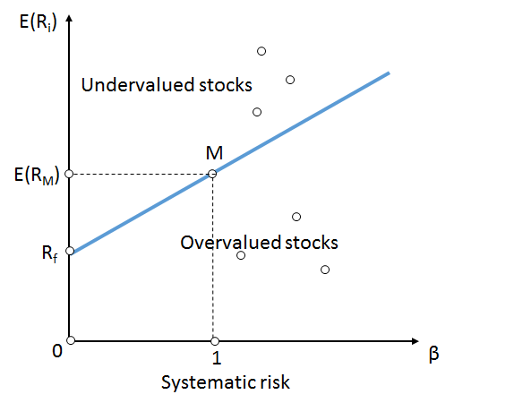
According to CAPM, the returns of low beta stocks were supposed to linearly scaled by their beta exposure, likewise with higher beta stocks. Instead, it was noticed that there was an unexpected curve:
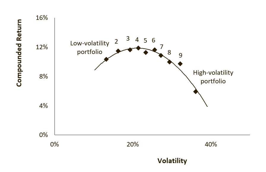
As we can see, high volatility (and thus, high beta) portfolios are returning significantly less than what is expected, thus throwing a wrench into the very concept of beta. After seeing the chart, a natural question is: can we exploit this mispricing while not being exposed to the market? In this post, we'll look into whether it's possible to profit off of this effect and also discuss the potential structural and behavioral reasons for this anomaly.
A Simple Approach
Of course, the simplest way to try and capture the excess return of the anomaly is to construct a portfolio of low beta equities and call it a day. But what if we don't want to be exposed to the market, even to the degree that low beta equities are? Like most answers in finance, the answer is a market neutral long/short portfolio!
For this strategy, we'll be using the Quantopian Q1500US universe, which consists of the 1500 most liquid US equities on any given day. We then construct our low beta factor as such:
\[f = \text{Z}[\text{rank}(-\beta_{252})]\]This will give us large positive values for stocks that have low beta, and small negative values for those that have high beta. Before we rank and z-score, in order to calculate the beta for each equity, we find the slope of a simple linear regression over a 252 day rolling window. We then use these factor values as the weights of our long/short portfolio. Let's look at the total long/short return of our simple strategy between 2003-01-01 and 2020-01-01:
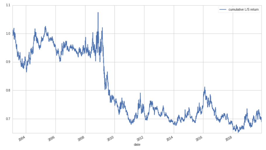
Well… this isn't good! Why are we losing money? Does this mean that the low beta anomaly isn't actually true? Digging into the numbers a little more, it turns out that the total portfolio beta for this strategy is actually negative, -38% to be exact. This means that even though we are market neutral, we have a negative exposure to the market: when the market goes up, our portfolio loses money, and vice versa. Since the market goes up most of the time, this isn't a great property to have. Ideally, we want to have zero beta exposure, not negative exposure. Let's look at the skew of the distribution of betas over time:
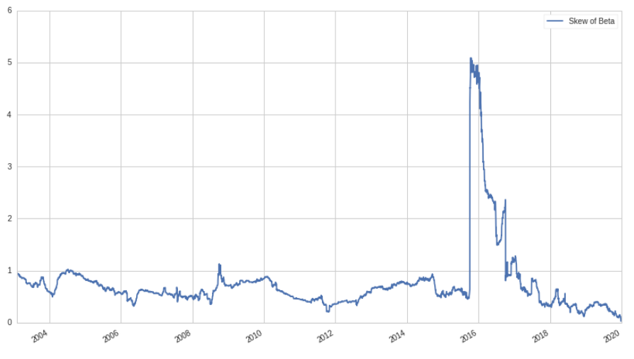
In order for our market neutral portfolio to have zero beta, we would need the skew of the betas to be zero, like for a standard normal distribution. To make this a little more concrete, let's look at a histogram for a single time period of stock betas:
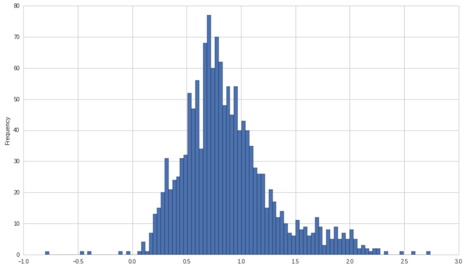
Now, the problem becomes evident: even though we are market neutral, we end up taking on negative beta exposure because the distribution of the beta of stocks has a long side-side tail. Almost no stocks actually have negative beta exposure, while many have high beta exposures! This means that when longing and shorting in equal proportion, we end up with a large negative beta since our long positions don't have a low enough beta in order to cancel out our high beta short positions.
Fixing the Problem
So, how do we proceed? We need to find some way to adjust the weights of our portfolio so that we end up with zero beta exposure. Fortunately, calculating the beta exposure is relatively straightforward. Given a column vector of weights:
\[\mathbf{X} = \begin{bmatrix} x_1 \\ x_2 \\ \vdots \\ x_n \\ \end{bmatrix}\]And a vector of beta exposures:
\[\mathbf{B} = \begin{bmatrix} \beta_1 & \beta_2 & \dots & \beta_n \end{bmatrix}\]We can easily find the beta of portfolio:
\[\beta_p = \mathbf{BX}\]Traditionally, we would solve this equation by using an optimizer with a constraint that $\beta_p =0$. But because we only have one factor, we can find an analytical solution. What we want to do is to try and solve for a $\beta_p$ of zero. To do this, we first need to rewrite the equation in terms of the weights that are positive (the low beta side) and those that are negative (the high beta side):
\[\mathbf{X_\alpha} = \begin{bmatrix} x_1 \\ x_2 \\ \vdots \\ x_j \end{bmatrix}\] \[\mathbf{X_\beta} = \begin{bmatrix} x_1 \\ x_2 \\ \vdots \\ x_k \end{bmatrix}\]Likewise, we split up the betas as well:
\[\mathbf{B_\alpha} = \begin{bmatrix} \beta_1 & \beta_2 & \dots & \beta_j \end{bmatrix}\] \[\mathbf{B_\beta} = \begin{bmatrix} \beta_1 & \beta_2 & \dots & \beta_k \end{bmatrix}\]Where:
\[n = j + k\]Now, our equation becomes:
\[\beta_p = \mathbf{B_\alpha X_\alpha}+\mathbf{B_\beta X_\beta}\]Where the $\alpha$ vectors contain the positive weights and the $\beta$ vectors, the negative weights. We want to scale up the negative weights (make them larger, though still negative), so we introduce a scaling factor, $\lambda$, and set $\beta_p=0$:
\[\mathbf{B_\alpha X_\alpha}+ \lambda \mathbf{B_\beta X_\beta}=0\]We now solve for $\lambda$:
\[\lambda = - \frac{\mathbf{B_\alpha X_\alpha}}{\mathbf{B_\beta X_\beta}}\]Assuming a leverage ratio of one, i.e:
\[\sum_{i=1}^j |x_{\alpha,i}| + \sum_{i=1}^k |x_{\beta,i}| = 1\]We can calculate the net long exposure, using $\lambda$ as a parameter:
\[l = \frac{1-\lambda}{1+\lambda}\]Below is the graph of net long exposure over time:
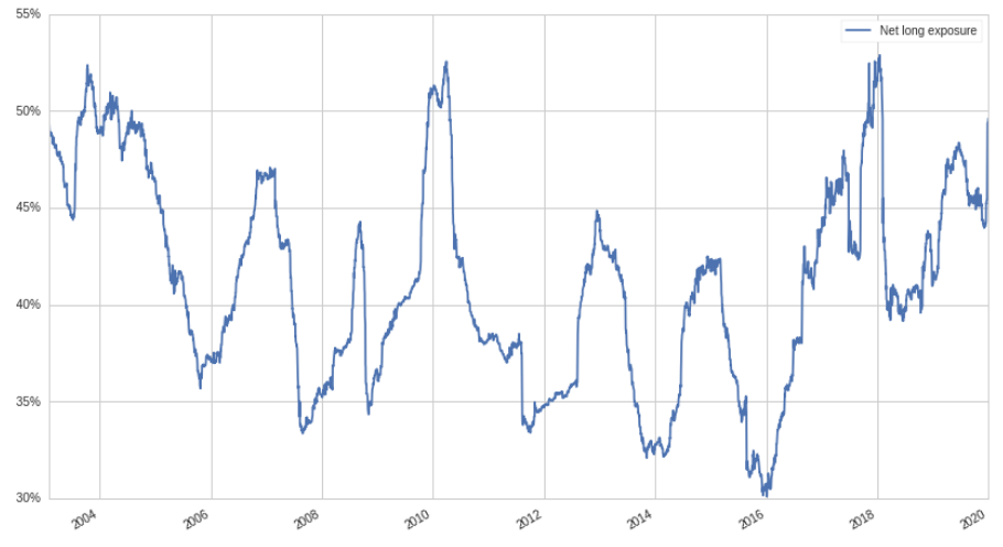
And the cumulative return:
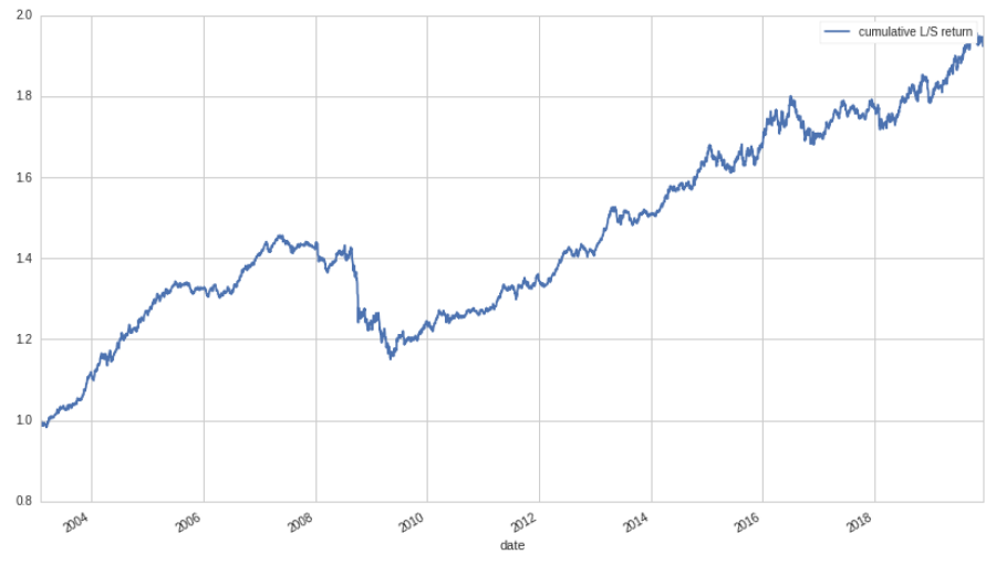
Wow, Looks a lot better! Ignoring the Great Recession, the return stream seems very solid, with limited volatility. Below is a table of some additional strategy information:
| Metric | Value |
|---|---|
| Beta | 1.8% |
| Ann. Ret | 4.0% |
| Ann. Vol | 4.6% |
| Ret/Vol | 0.84 |
With a beta of only 1.8%, it's clear that our method for reducing beta exposure works quite well. Still, it's surprising that a net long exposure of such magnitude can still be taken with little to no correlation to the market. Evidently, there is indeed an excess return associated with low-beta equities, and quite a large one, at that.
Explanation
Many academics have tried to explain the structural and behavioral reasons for the low beta anomaly. The most common explanation put forth is that due to leverage constraints and borrowing costs, investors seek out high beta securities in order to achieve a higher natural return. If high leverage ratios were available to all investors, one might expect that this mispricing of high beta stocks might go away, as the beta of any given stock would become less important.
Another possible explanation is that the conflict of interest between money managers and clients creates an incentive for fund managers to take excess risk through high beta equities. In good times, managers collect a performance fee and a management fee while in bad times, only a management fee. This asymmetric payoff incentives managers to try and score a big "win," while limited liability prevents managers from ever losing money on losses.
A third explanation is that high volatility (and thus high beta) stocks receive more attention from the financial community as they are simply more interesting to discuss. This interest and attention encourages increased buying, thus pushing down the expected return of said stocks.
Conclusion
In this post we have shown that there is indeed a significant abnormal return associated with low beta stocks. This abnormal return can not only be captured with a long only (and beta exposed) portfolio, but also a beta neutral one. Despite the less than stellar risk-adjusted return of the strategy, perhaps the Sharpe ratio can be improved by controlling sector and style risks in addition to beta exposure. Perhaps one could also overlay the low beta factor on top of an existing factor strategy in order to reduce volatility and boost the risk-adjusted return.
That's all for now, and thanks for reading! If you're interested in the code and want to play around with it, check it out here.