In part one, we looked into the relationship between volatility, returns, and leverage and derived an equation for the optimal leverage ratio that maximizes the expected return of a portfolio. This leverage ratio is dependent on two principle components, expected variance and expected returns:
\[l = \frac{r_b}{\sigma^2_b}\]Where $r_b$ is the unlevered return and $\sigma^2_b$, the variance of the portfolio. Our next task, though clear, is hardly straightforward: we must forecast the future expected return and volatility of the portfolio in order to set an appropriate leverage ratio. In Part three, we'll use our forecasts developed in this post, with modifications and extensions, to realize a complete trading strategy that attempts to deliver a higher return than the market through the application of variable leverage.
Autoregressive Model
There are an unaccountably numerous number of modeling techniques that attempt to do time-series forecasting, each of varying complexity and sophistication. To start off with, let's consider a moving average (AR) model:
\[\text{AR}(p): x_t = \alpha + B_1x_{t-1}+B_2x_{t-2}+\cdots+B_px_{t-p}+\epsilon_t\]Simply put, an AR model is simply a multiple regression on previous observed values with the addition of a white noise component. Values of $x$ come from previous observed values in the series. For example, a model that simply used today's returns as a predictor for tomorrow's returns could be approximately formalized as a AR(1) model with $\alpha=0$ and $B_1=1$:
\[\text{AR}(1): x_t = x_{t-1} + \epsilon_t\]Note that $\epsilon_t\sim N(0, \sigma^2)$, which means it is a white noise term with a mean of zero and a standard deviation that equals the volatility of the time series in question.
There are various ways to find an appropriate $p$, but perhaps the most straightforward is to apply the autocorrelation function, also called ACF. The ACF takes in a number that represents the number of previous values we are interested in and calculates the correlations over the different lagged values. For example, if we wanted to find the ACF with a lag of one, we would simply find the correlation between all values (except the first one), and the previous value in the time series. By calculating the ACF over a number of lags, we can discover if there is a serial correlation between values or if they are independent. For example, if we found that there is a correlation, positive or negative, between today's market returns and the returns of yesterday, but not the day before yesterday, we could use an AR(1) model to capture this relationship.
Moving Average Model
Another type of simple model often used to forecast time series is an autoregressive or AR model:
\[\text{MA}(q):x_t = \mu + \epsilon_t + \theta_1\epsilon_{t-1}+\cdots+\theta_q \epsilon_{t-q}\]A MA model is defined by its lag, $q$, the number of previous terms to consider when generating a forecast. Each future forecast in parameterized by the mean, which must remain constant and $\theta_1\cdots\theta_q$, the lag exposures. $\epsilon_{t-q}\cdots\epsilon_t$ are lagged white noise terms generated from previous observations. These epsilon error terms are unobservable, independent of each other, and respect a normal distribution. It is important to note that because $\mu$ is constant, the time-series in question must be stationary: the mean and variance must not change over time.
Instead of using the ACF to discover the serial correlations and the $q$ parameter, we use the partial autocorrelation function (PACF) instead. The PACF is similar to the ACF, except that it calculates the partial correlation instead of a regular correlation over lagged values. Partial correlation differs in that it controls for some specified variable before the correlation function is run. In the case of PACF, we control for the linear dependence of the non-lagged values with the values in between. For example, let's say we're looking at the PACF of lag 2 and have three variables to consider: $x_t$, $x_{t-1}$, and $x_{t-2}$. The partial autocorrelation is the same as normal correlation between $x_t$ and $x_{t-1}$. But when considering $x_t$ and $x_{t-2}$, we first remove the dependence that $x_t$ has on $x_{t-1}$ before running the correlation.
ARIMA Model
A common approach is to combine both of these models, forming an ARMA model:
\[\text{ARMA}(p,\,q): \text{AR}(p) + \text{MA}(q)\]Note that an ARMA model is only appropriate when the series is stationary, the mean and variance must not change over time. Because of this, such a model is inappropriate for the forecasting of price data, instead returns must be used. What we're implicitly doing is differencing the price series, also called integration of order one. An ARIMA (autoregressive integrated moving average) model captures this differencing:
\[\text{ARIMA}(p,\,d\,,q)\]Where $d$ is the number of times we differenced. This implies that ARIMA(1, 1, 1) on price data is identical to ARMA(1, 1) on return data:
\[\text{ARIMA}(p,\,1,\,q) p_t = \text{ARMA}(p,\,q) r_t\]Also note that:
\[\text{ARIMA}(p,\,0,\,q) = \text{ARMA}(p,\,q)\]In order to find an appropriate $d$, wee can use the Augmented Dickey Fuller (ADF) test to iteratively determine the integration order necessary. The ADF test produces a p-value indicating the probability that the series is not stationary. The process for determining the integration order and therefore $d$ for an ARIMA model might look as follows:
- Set $d=0$
- Apply the ADF test on the series
- If $p\leq0.05$, return $d$
- Otherwise, take the difference between each successive value and increment $d$.
- Go to step 2
Forecasting Returns
Now that we've covered some background on time series forecasting, let's jump into it: predicting the future return. We will be using an ARMA instead of an ARIMA model, as in general, returns are stationary over long periods of time. First, we should look at the ACF output so we can find a good $p$. Different return windows might exhibit different serial correlations, so let's look at the ACF of one day, one week, and one month returns between 2003-01-01 and 2020-01-01:
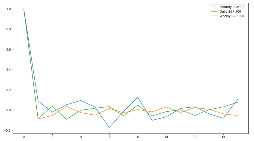
It definitely seems that both weekly and daily data do not exhibit very much, if any, serial correlation between subsequent periods. Monthly returns, on the other hand, exhibit a weak correlation between adjacent months. From this graph, a $p$ of 1 is probably the most appropriate value.
Moving on to the PACF, we observe much the same results as before:
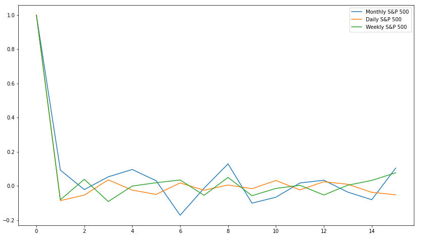
This isn't surprising, as over short lag periods with low correlation to each other, the PACF should look relatively similar to the ACF. As before, we'll decide on a $q$ of 1.
In order to avoid lookahead bias, we will use a starting window value of 96 months, or 8 years. For each subsequent month, we will add the observation and then refit our ARMA parameters. This means that our window increases by one every single iteration: on our second to last observation, we are using almost all of the available data to train the model. Another possible approach would be to use a constant rolling window, though we would have to take care to ensure that each window was stationary. A third approach would be to use some percentage of the data for fitting parameters and the rest for validation, but an increasing window ensures that new data is always used for fitting as it is made available. Below is the graph of the forecasted versus actualized return for the S&P 500:
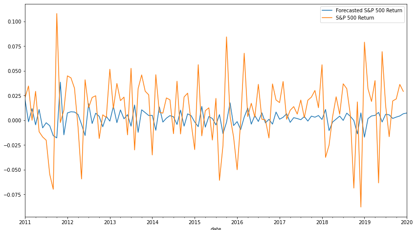
Though not exceptional, the model does get the direction of the return (either up or down) right 55% of the time: not terrible for a simple and straightforward model. It's also evident that the model significantly underestimates the volatility of the market, with the magnitude of predicted returns being quite modest. This is unsurprising for several reasons: market returns exhibit excess kurtosis compared to a normal distribution, and the residuals must also follow a normal distribution. All in all, this is a decent start, especially considering that predicting returns with a high accuracy is a notoriously difficult, and perhaps intractable, problem.
VIX Index
Now that we have the foundations of the return model out of the way, we can move onto to the volatility component. Two principle methods of forecasting volatility are commonly used: the VIX and GARCH. Let's first discuss the VIX.
By using the implied volatility of S&P 500 calls and puts, the VIX index aims to predict the one month volatility of the market. By using the current price of puts and calls for the S&P 500, we can use the Black Scholes options model to solve for the implied volatility, or the future volatility necessary to justify the current prices. At the time of writing, the VIX index currently is at 28.59. This means that the future expected one month annualized volatility is 9.9% or the square root of 12 multiplied by 2.859%. Unfortunately, using the VIX as a measure of future volatility has some problems: because options are primarily used to hedge downside risk, the VIX often underestimates the future upside volatility and overestimates the future downside volatility.
In a strong bull market, call options are often undervalued, as there are other, more common ways to express a long view on the market, such as futures or equities. During bear markets, put options become overpriced as they are one of the only ways to hedge a portfolio without assuming unlimited price risk (such a shorting or selling futures). The consequence of this is that the VIX often serves as nothing more than an index that represents the inverse of market returns: when the market goes up, the VIX goes down, and vice-versa. Below are two graphs of the correlation between the VIX and future one month volatility and previous volatility and future volatility:
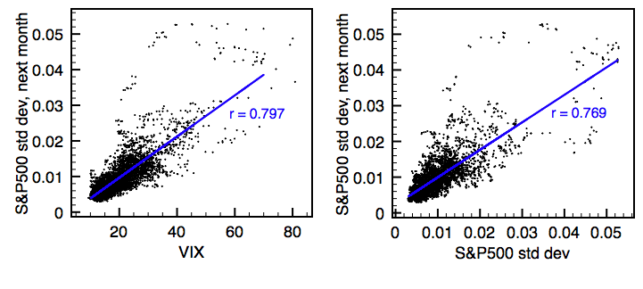
Perhaps surprisingly, the VIX has practically the same predictive power as simply using last month's volatility.
GARCH Model
Instead of using the VIX, we are going to use an Generalized Autoregressive Conditional Heteroskedasticity (GARCH) model. GARCH is more complicated than ARIMA, so we won't get into the mathematics of how it works, but, in short, GARCH allows for the volatility to experience "shocks" through time. The output of a GARCH model is the conditional volatility: the instantaneous volatility with respect to some model. One can think of the conditional volatility as the unobservable latent volatility that changes over time. Unlike traditional volatility, which must be calculated over some time window, conditional volatility exists at an instantaneous point of time. Though we're not going to talk about GARCH parameters in this post, for those that are already familiar with GARCH, note that we are using the standard GARCH(1, 1) model, the most common parameters for forecasting the volatility of returns.
Forecasting Volatility
Unlike with our ARMA model, we are going to using the daily instead of monthly returns of the S&P 500 for our GARCH model. Much like before, we are going to take an ever expanding window, starting at 63 days or 3 months. Also like with returns, by the penultimate observation, we will be using almost all available data for training our model. The following graph is of annualized conditional volatility vs the annualized 21 day (one month) volatility:
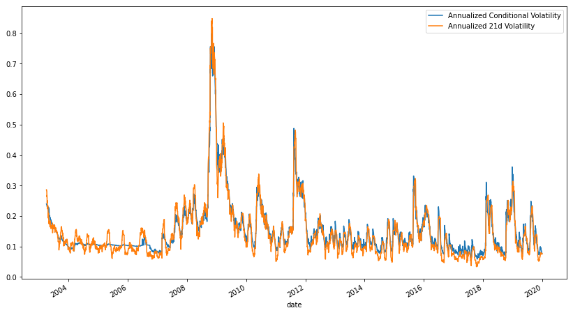
Just from the graph, the accuracy of our model looks very good. And in fact it is, with a correlation of 97.6% and a Mean Absolute Percentage Error (MAPE) of only 14.8%. All things considered, this is quite good and highlights the incredible predictive power of GARCH models in forecasting volatility.
Conclusion
Now that we have a monthly model for forecasting returns and a daily modal for forecasting volatility, we conclude this blog post. Modifications will need to made to turn this into a real, long-only S&P 500 ETF, but a good foundation has been laid. I hope you enjoyed this post! Click here to check out the notebook. If you install anaconda, no additional Python libraries should be necessary to execute the notebook.